Mastering DC-DC Efficiency with SSA Modeling in Keysight ADS

Benjamin Dannan
Mar 5
11 min read

The Imperative of DC-DC Converter Efficiency

In today's ever-more power-conscious electronic world, the efficiency of power delivery networks is paramount. From the smallest battery-powered IoT device to the largest data center server, every milliwatt saved translates directly into extended battery life, reduced operating costs, and enhanced system reliability. At the heart of these power delivery networks often lie DC-DC converters, specifically Voltage Regulator Modules (VRMs), which play a critical role in transforming input voltages to the precise levels required by high-performance integrated circuits like CPUs, GPUs, and FPGAs. This blog post will delve into the critical importance of DC-DC converter efficiency, explore when this metric becomes a design imperative, highlight applications where its simulation is indispensable, and ultimately demonstrate how our advanced State-space average VRM models within Keysight ADS provide a powerful solution for accurate and efficient efficiency analysis. If you're looking for DC-DC converter simulation tools, understanding this approach is key to answering the core question: how to calculate VRM efficiency accurately in a virtual environment.

Why Does Every Percentage Point of VRM Efficiency Matter?

What is Power Supply or DC-DC Converter Efficiency?

At its core, the efficiency of a power supply or DC-DC converter is a measure of how effectively it converts input electrical power into usable output electrical power. Expressed as a percentage, it's defined by the ratio of output power (Pout) to input power (Pin):

Efficiency(η)=Pout/Pin×100%

The difference between input and output power represents the power lost within the converter, primarily dissipated as heat. These losses arise from various sources, including:

Switching Losses: Occurring during the ON/OFF transitions of switching elements (MOSFETs, IGBTs), these losses are proportional to switching frequency, gate charge, and voltage/current overlap.
Conduction Losses: Due to the ON-state resistance (RDS(on)) of switching devices and the equivalent series resistance (ESR) of inductors and capacitors. These are proportional to the square of the current (I2R).
Gate Drive Losses: Power consumed by the circuitry that drives the gates of the switching elements.
Magnetic Losses: Hysteresis and eddy current losses within inductors and transformers.
Quiescent Current/No-Load Losses: Power consumed by the control circuitry and other internal components even when no load is present.

This example addresses the main power loss mechanisms, but other losses can be added if higher fidelity is required.

A "good" DC-DC converter typically boasts efficiencies exceeding 90%, and for many applications, designers strive for 95% or even higher.

When is this Metric Useful and Why is it Important?

The significance of high efficiency extends across several critical domains:

Thermal Management and Reliability: The most direct consequence of inefficiency is heat generation. Higher losses mean more heat, which must be dissipated by cooling solutions (heatsinks, fans, etc.). Excessive heat directly impacts the lifespan and reliability of electronic components. According to the Arrhenius relationship, chemical reaction rates (and thus aging and failure rates) approximately double for every 10°C increase in temperature. A more efficient VRM (or voltage regulator) generates less heat, leading to a cooler-running system and significantly extending its operational life. This also reduces the complexity and cost of thermal management solutions.
Energy Consumption and Operating Costs: In systems that run continuously or in large quantities (e.g., data centers, industrial equipment), even a few percentage points of efficiency improvement can translate into substantial energy savings and reduced electricity bills over the product's lifetime. For instance, a 1kW power supply with 94% efficiency wastes 60W, whereas a 96% efficient supply wastes only 40W. Over a year, this seemingly small difference can amount to hundreds of kilowatt-hours (kWh) of wasted energy, easily exceeding the initial cost of the power supply itself. High VRM efficiency directly contributes to improved overall system performance and power usage effectiveness (PUE) in large facilities.
Battery Life and Portability: For battery-powered devices like smartphones, laptops, IoT sensors, and wearable electronics, efficiency is paramount. Every joule of energy conserved directly extends battery runtime, a key differentiator in the consumer market. Higher efficiency allows for smaller batteries, reducing device size, weight, and material costs.
Power Density and Miniaturization: As electronic devices become smaller and more integrated, there's a constant drive to increase power density (power delivered per unit volume). Higher efficiency means less heat generation for a given power output, allowing designers to pack more functionality into a smaller footprint without compromising thermal limits. This is crucial for compact designs in mobile, automotive, and aerospace applications.
Compliance with Energy Standards: Governments and regulatory bodies worldwide are increasingly imposing stringent energy efficiency standards (e.g., 80 PLUS certification for PC power supplies, various international efficiency marking protocols). Designing for high efficiency from the outset is essential to meet these requirements and gain market access.

Which High-Performance Applications Require VRM Efficiency Simulation?

The ability to accurately simulate VRM efficiency at the design stage is a game-changer for a wide range of applications:

High-Performance Computing (HPC) and Data Centers: CPUs, GPUs, and specialized accelerators in servers and data centers consume significant power. Maximizing VRM efficiency is vital to minimizing operating costs, reducing cooling requirements, and improving the overall power usage effectiveness (PUE) of data centers.
Automotive Electronics: Electric Vehicles (EVs) and Hybrid Electric Vehicles (HEVs) rely heavily on efficient DC-DC converters for power management across various voltage domains (e.g., 400V or 800V bus to 12V battery, traction inverters). High efficiency is critical for extending range, reducing battery size, and managing thermal loads in confined spaces. Achieving high EV DC-DC converter efficiency is now a primary design goal. Bidirectional DC-DC converters, in particular, demand high efficiency in both buck and boost modes.
Consumer Electronics: Smartphones, tablets, laptops, gaming consoles, and smart home devices all benefit immensely from efficient power conversion to extend battery life and reduce heat in compact designs.
Industrial and Telecom Infrastructure: Power supplies for base stations, industrial control systems, and power tools require robust and efficient VRMs to ensure reliable operation, minimize downtime, and reduce energy consumption in always-on environments.
Medical Devices: Wearable and implantable medical devices often have extremely tight power budgets. Highly efficient DC-DC converters are essential for maximizing battery life and minimizing heat generation in sensitive applications.
Aerospace and Defense: Weight and thermal management are critical in aerospace applications. Efficient power converters contribute to lighter systems and simpler cooling, enhancing mission duration and reliability. The goal here is always to achieve high correlation in the VRM simulation vs datasheet performance before physical prototyping.

How Do State-Space Average VRM Models Accelerate Efficiency Analysis?

Traditional transient simulations of switching power supplies can be computationally intensive and time-consuming, especially when trying to analyze efficiency across a wide range of operating conditions. This is the challenge engineers face when performing a transient vs state-space simulation comparison where the Sandler State-space average (SSA) VRM models in Keysight ADS revolutionize the design process.

State-space averaging is a powerful modeling technique that provides a simplified, yet highly accurate, representation of a switching power converter. Instead of simulating the fast, cycle-by-cycle switching behavior, SSA models average the behavior over a switching period, allowing for significantly faster simulations without sacrificing fidelity for small-signal AC and large-signal transient analysis relevant to efficiency. This provides a truly fast VRM model for PDN analysis.

Key advantages of using our Sandler State-space average VRM models in Keysight ADS for efficiency simulation include:

Accelerated Simulation Speed: By abstracting away the high-frequency switching details, SSA models dramatically reduce simulation time, enabling designers to perform extensive parametric sweeps and corner analyses for efficiency optimization in minutes rather than hours or days.
Accurate Loss Mechanisms: Advanced SSA models, such as the Sandler State-Space Average Model, can accurately capture various loss mechanisms (switching losses, conduction losses, gate drive losses, etc.) as a function of operating conditions (input voltage, output current, duty cycle, switching frequency). This allows for a precise calculation of efficiency across the entire load range.
Comprehensive Power Integrity Analysis: Keysight ADS, with its robust simulation capabilities, allows for the seamless integration of SSA VRM models with other power delivery network (PDN) components (PCB traces, decoupling capacitors, IC package models, die models). This provides an end-to-end power integrity simulation environment, enabling designers to understand how VRM efficiency interacts with the broader PDN and impacts overall system performance, including ripple and transient response.
Early Design Optimization: Simulating efficiency early in the design cycle allows engineers to evaluate different VRM topologies, component choices (MOSFETs, inductors, capacitors), and control strategies, enabling rapid iteration and optimization for peak efficiency before committing to hardware prototypes. This proactive approach significantly reduces design cycles and development costs.
Sensitivity Analysis and Tolerancing: With fast simulation, designers can easily perform sensitivity analyses to understand how variations in component parameters (e.g., RDS(on) tolerance, inductor DCR tolerance) affect overall efficiency, enabling robust design for manufacturing.

In the upcoming sections of this blog, we will walk through practical examples in Keysight ADS, demonstrating how to set up and run simulations using our State-space average VRM models to extract critical efficiency data. Get ready to unlock new levels of power design optimization!

How to Set up an Efficiency Simulation in Keysight ADS

After adding the Sandler State Space Average Converter model from the SES model library to your schematic, you will need to set up your VRM, regulator, or buck converter circuit for simulation. This video HERE shows how to get started with our SI/PI library in ADS. For this example, we will use the Texas Instruments TPS62818-Q1 converter.

The TPS62816-Q1 is a pin-to-pin high-efficiency, easy-to-use synchronous step-down DC/DC converter. It is based on a peak current mode control topology. It is designed for automotive applications such as infotainment and advanced driver assistance systems. Low-resistive switches allow up to 6-A continuous output current.

The circuit in Figure 1 demonstrates how to simulate efficiency with a 5V input and a 1.8V output. Notice on the TPS62816-Q1 model, we have two outputs depicted, a large signal output and a small signal output. For this simulation, we only need to use the small signal output. We will use an I_DC source to sweep our output load current, which is depicted by SRC6. After setting up your circuit, add a current probe at the input and output of the regulator, as shown below. You can see we have named these "I_Probe_vin" and I_Probe_vout" respectively.

To simulate efficiency, we will use a DC simulator in ADS and add a parameter sweep. If you'd like a more granular sweep option, you can also add a sweep plan, as shown in Figure 1 below.

Figure 1 - Example Keysight ADS Efficiency Simulation with the TPS62816-Q1 Converter

How to Set Up the Load Current Sweep in Keysight ADS?

An example of how to set up our DC simulation, with a parameter sweep and a sweep plan in Keysight ADS, is shown in Figures 2 and 3. A sweep plan is not necessarily required unless a more granular sweep is desired. Generally, an efficiency simulation can be achieved with only a parameter sweep.

In this example, we are sweeping the "I_load" variable, which is the DC current on our current source shown in Figure 1 by SRC6.

Figure 2 - Keysight ADS DC Simulation Set up with Parameter Sweep and Sweep Plan

Figure 3 - Keysight ADS Sweep Plan Setup Example

Setting up the Data Display

After running your simulation, we need to add some equations to our ADS data display before plotting the efficiency curves.

For our current probes, the vin and vout_ss nodes (shown in Figure 1), we need to note that these are arrays that contain multiple responses for each swept current value. So our arrays are 2 columns each—one for the array index and the other for the respective array value at the array index.

The equations shown below detail how to calculate our VIN, Iin, Vout, Iout, Input power, output power, and lastly our efficiency.

VIN, Iin, Vout, Iout, Input power, output power, and efficiency equations

As the next step to plot our efficiency, we need to add a plot to our data display and add the following trace expression, as depicted in Figure 4.

Trace Expression: plot_vs(EFF_ss_dc, Iout_ss_dc)

Figure 4 - Data Display Trace Expression Example for Efficiency versus Output Current

Our efficiency results are shown below in Figure 5, in comparison to the TI datasheet, specifically Figure 10-5, which details a result for a 1.8V output. After a quick observation, we can see our result for 5Vin does not match up well at all with the datasheet. Why is that?

Figure 5 - TPS62816-Q1 Datasheet vs. Simulated Efficiency without Inductor Core Losses

The answer is straightforward, in that we need to remember that inductor power loss is broken down into two parts, the DC loss and the AC loss. If you reference some Coilcraft articles and MuRata's Power Inductor Course - Chapter 3, you will find more details on this topic. In short, the hysteresis effect is one of the main sources of loss in ferromagnetic materials, or inductors, which must be accounted for to achieve accurate simulation results. This is where the Steinmetz Equation is used. However, there are online tools that provide this estimated loss, which we will discuss shortly. This is an important area where tips for simulating power converter loss can make a huge difference in accuracy.

As per MuRata's Power Inductor Course, DC loss is proportional to Rdc (direct current resistance) because it is the conductor power loss from a direct current passing through a coil of wire. Meanwhile, AC loss is proportional to Rac (alternating current resistance) and is defined as the power loss in the conductor from an alternating current passing through a coil of wire. AC loss includes power loss in the core, which is also referred to as iron loss. At high frequencies, power loss in the conductor also tends to increase due to the skin effect.

So, now, how do we determine our DC and AC power loss?

Well, our DC power loss is a function of the inductor's DCR value and the current through the inductor.

To determine the AC power loss, we will use the Coilcraft Power Inductor Analyzer. From this tool, we can calculate our AC and DC power loss in our inductor. An example of this result is shown in Figure 6 for the XGL4020-251 (250 nH) inductor, which is used in this example.

Figure 6 - Coilcraft Power Inductor Analyzer - XGL4020-251 (250 nH) inductor Result @ 6A

From this Coilcraft analyzer, we can plot our AC and DC loss at our switching frequency (2.25 MHz) for multiple DC currents as shown in the Table below.

Table 1 - Coilcraft Power Inductor Analyzer AC Loss Results for XGL4020-251 (250 nH) inductor

Using this average Rac value of 2.8 mOhm and the DCR value of 2.5 mOhm, we can plot the inductor DC and AC power losses, which are depicted in Figure 7. We observe that the AC loss is 101 mW at 6 A, close to the value found (119mW) in the table above, using the Coilcraft Analyzer tools shown in Figure 5. This is a significant term that needs to be included in our efficiency calculation, and this demonstrates why we previously did not have a good correlation with the manufacturer's datasheet.

Figure 7 - Coilcraft XBL4020-251 Inductor DC and AC Power Loss versus Output Current

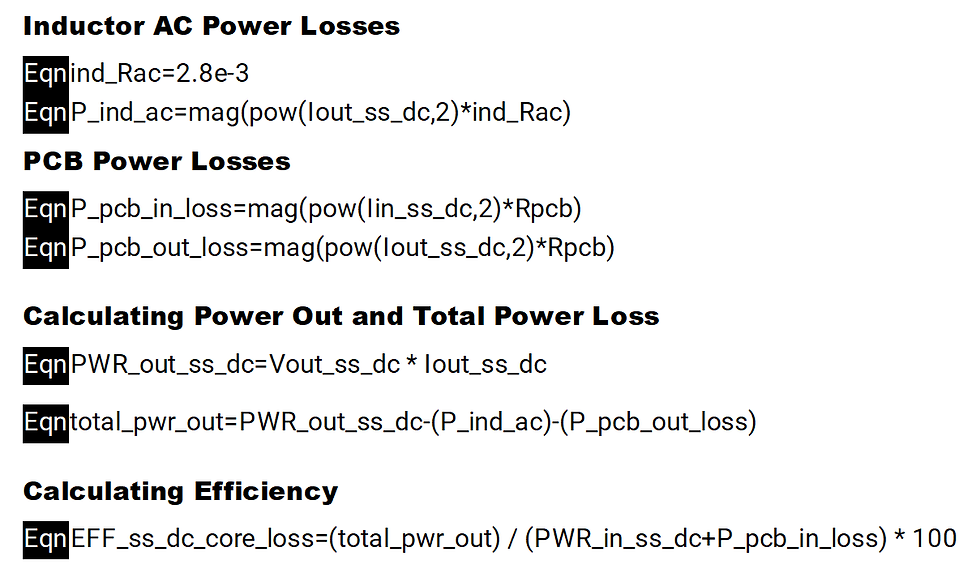
Now, let's account for these inductor AC losses in our efficiency equations, which are shown below.

Having accounted for both the inductor AC loss and additionally, the PCB loss in our equations, as displayed in the ADS data display equations below, we can now calculate a more accurate efficiency result, shown in Figure 8. In this example, our PCB loss is based on a PCB resistance of 6 mOhms. This number was found by fitting our simulated model to the datasheet result after accounting for the inductor AC losses.

When comparing this updated simulated result to the datasheet, we can see that our simulated result correlates much more closely with the datasheet. This high correlation between VRM simulation vs datasheet confirms the validity of the modeling approach. Using this method provides an accurate and fast solution to simulate power supply efficiency for your designs.

Figure 8 - TPS62816-Q1 Datasheet vs. Simulated Efficiency with Coilcraft XGL4020-251 Inductor Core Losses

Conclusion: Achieving Accurate VRM Efficiency Results

In this blog, we discussed why efficiency is important and showed a detailed, accurate example of how to simulate efficiency with inductor DC and AC losses using our Sandler State-Space Average VRM models. Furthermore, with this modeling method, if desired, designers can model the efficiency of an entire power system, which could include multiple cascaded regulators. If you're interested in conducting more accurate simulations or learning more about our ADS VRM models, check out our SI/PI library HERE, and please don't hesitate to reach out.

If you want to learn more about how you can co-simulate with our ADS VRM models, check out this BLOG.

If you're looking for support within your team for signal integrity or power integrity simulation, please reach out to us at the email (info@signaledgesolutions.com) or through our website.